Loading
Welcome

Welcome to the Interactive Catchment Explorer (ICE), a web-based data visualization tool for exploring complex, multivariate environmental datasets and model results. It is designed to help researchers and resource managers identify spatial patterns in hydro-ecological conditions and to prioritize locations for restoration or further study.
This application contains the following datasets and models:
- Northeast Catchment Delineation: a custom, high resolution catchment delineation and basin characteristics dataset of the Northeast U.S.
- Northeast Stream Temperature Model: a hierarchical Bayesian model for predicting daily mean stream temperature using observed data from the Northeast Stream Temperature Database.
- Northeast Brook Trout Occupancy Model: a logistic mixed-effects model for predicting the probability of Brook Trout occupancy based on predicted stream temperatures under historical and potential climate change scenarios.
More information about the datasets and models can be found by clicking the Datasets button on the upperleft toolbar.
Disclaimer: The models used in this project were designed to capture large-scale, regional patterns in stream temperature and brook trout occupancy. Although results can be viewed at the local catchment scale, the accuracy of these models can vary widely from catchment to catchment depending on the amount of available local data and other factors. Please use caution when interpreting the results at local spatial scales.
Other Versions: ICE has been adapted for a variety of other datasets and models around the country. Other versions of ICE can be found at https://usgs.gov/apps/ecosheds.
Citation: Walker JD, Letcher BH, Rodgers KD, Muhlfeld CC, D'Angelo VS (2020). An Interactive Data Visualization Framework for Exploring Geospatial Environmental Datasets and Model Predictions. Water 12(10):2928. https://doi.org/10.3390/w12102928
Team: ICE is part of the EcoSHEDS project and was developed by Dr. Jeffrey D. Walker (Contractor to USGS, Walker Environmental Research) and Dr. Benjamin Letcher (USGS, Eastern Ecological Science Center).
Funding: This project was funded by the NE Climate Science Center, North Atlantic Landscape Conservation Cooperative, USGS and DOI Hurricane Sandy Restoration funds, and the USGS National Climate Science Center.
User Guide
Overview
The Interactive Catchment Explorer (ICE) is a data visualization tool for exploring environmental datasets and model outputs.
ICE is designed to:
- Identify spatial patterns of hydro-ecological conditions over a wide range of scales,
- View and compare the distributions (histograms) of selected variables and regions,
- Use interactive cross-filtering to identify areas that meet one or more specific criteria and to discover correlations and relationships between variables.
Dataset Options
The dataset being shown on the map is controlled by three sets of options, which are configured using dropdown menus.
The Resolution option determines the set of HUC* basins that are used to spatially aggregate the individual catchments (see Spatial Aggregation below). Higher values correspond to the higher resolutions (HUC6 is the lowest resolution, HUC12 is the highest). Due to the large number of HUC12 basins across the Northeast, this resolution is divided into 2-digit HUC sub-regions, only one of which can be viewed at a time (see HUC2 map).
The States option allows you to focus on one or more states by filtering the dataset for only catchments within those states. For example, selecting only "Massachusetts" will filter the dataset to only include catchments located within Massachusetts.
The Variable option determines which variable is spatially aggregated and used to color-code each HUC. When this variable is changed, the legend will automatically update to reflect the range of values for the selected variable.
* HUC stands for Hydrologic Unit Code, which is a hierarchical drainage basin classification system developed by the USGS and USDA-NRCS commonly used for identifying distinct watersheds across the U.S.

Map Controls and Layers
The map provides a basemap (satellite or street map) and one or more static layers (streams, waterbodies, HUC boundaries). On top of the basemap and static layers is an interactive layer containing HUC basins for the selected resolution (e.g. HUC8, HUC10, etc.).
Map Controls
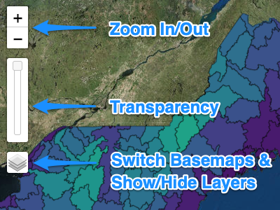
Use the map controls to zoom in and out, adjust the transparency of the HUCs, and switch basemaps or show/hide individual static layers.
The static layers (e.g. streams) are tiled images, and therefore not interactive (i.e., you cannot click on a stream to see more info).
HUC Basin Layer


The HUC basin layer shows the drainage areas for the selected resolution (see Dataset Options above).
The color of each HUC represents the average value of the selected variable among all catchments within that HUC (see Spatial Aggregation below).
Hover your mouse over a HUC to view its ID, name, and value for the selected variable.
Click to select a HUC. This will open a new toolbar showing the name and ID of the selected HUC, and provide additional tools to view the Data for all variables, Zoom To, view Catchments within, or Unselect that HUC.
Color Legend
The legend shows the color scale corresponding to the range of values for the selected variable.
Click the Legend Options link to open addition controls. The Colors menu provides alternative color scales. The Transform menu provides alternative variable transformations (i.e., linear or log). The logarithmic transformation can be useful for variables that exhibit a highly skewed distribution.

Spatial Aggregation

One of the primary goals of ICE is to allow users to explore large geospatial datasets. With nearly 400,000 catchments across the Northeast region, it would not be possible to provide an interactive layer with all of the catchments due to the memory and processing power required. To solve this problem, ICE spatially aggregates the individual catchments to larger HUC basins. This aggregation yields a smaller dataset (i.e., fewer polygons) that can be more efficiently displayed as an interactive layer on the map.
The spatial aggregation can be performed at varying HUC resolutions by changing the Resolution (see Dataset Options section above). By changing this resolution, users can compare patterns at varying spatial scales ranging from the local sub-basins (HUC12s) within a sub-region to the major drainage basins (HUC6s) across the entire Northeast region.
There are two ways the catchments can be spatially aggregated to the HUC basins depending on which option is selected from the Variable dropdown menu:
- % Area Filtered: If this option is selected, then the value for each HUC is the percent of the total area comprised of catchments that meet the filter criteria (see Histogram and Cross-filters below). For example, if a filter is set for elevation < 200 m, then the value of each HUC is the percent of the total area covered by catchments with elevations less than 200 m. When no filter is set, then all HUCs will have a value of 100%.
- Area-weighted Mean: If any of the other variables are selected, then the value for each HUC is the calculated using the mean of the filtered catchments within that HUC and weighted by catchment area. The area-weighted mean thus corrects for differences in the areas of the individual catchments within each HUC. For example, if the selected variable is Elevation (m), then the color of each HUC reflects the area-weighted mean elevation of the catchments within it. If one or more filters are set, then this value is computed only from the catchments that meet the filter criteria.
Histograms and Cross-filters
Histograms can be added on the right-hand side of the application to view the distribution of catchment values for one or more variables. These histograms also act as interactive filters (a process called cross-filtering), which allows you to focus on subsets of the data defined by one or more criteria. The cross-filters are responsive to user inputs, allowing the user to explore spatial patterns of individual variables interactively, as well as the relationships between variables as will be explained below.
Histogram of All Catchments

Select one or more variables from the drop down menu to open the corresponding histogram(s). Each histogram shows the distribution of values for all catchments in the region (assuming no filters have been set as explained below). The vertical blue line shows the mean value of the distribution.
The histograms show the distribution of the catchments, not of the aggregated HUC values.
Histogram of Selected HUC

When a HUC is selected, a secondary histogram (colored orange) shows the distribution for catchments within that HUC. This histogram can be compared to the primary (blue) histogram to compare the catchments within this HUC relative to all catchments across the entire region.
The primary (blue) and secondary (orange) histograms do not share the same y-scale. They are normalized in the y-dimension so that they have the same height, but may have different maximum counts (y values).
Filtering

Click and drag over a histogram to set a filter for that variable. This action will filter the data to a subset containing only catchments within that filter window. When a filter is set or changed, the spatially aggregated value of each HUC will be re-computed using only the filtered catchments.
For example, if a filter is set on Elevation (m) for all values greater than 200 m, then only catchments with elevations > 200 m will be used for the spatial aggregation. If the selected Variable is % Area Filtered, then the value of each HUC will reflect the % of the total HUC area containing the filtered catchments (e.g. 50% if half of the HUC area has catchments with elevations > 200 m). If any other variable is selected, then the value of each HUC will correspond to the area-weighted mean computed only from the filtered catchments with elevations > 200 m.
To reset (or clear) a filter, click the Reset link or simply click anywhere outside the current filter range on the histogram itself.
Setting Multiple Filters

Multiple filters can be set simultaneously by selecting more than one variable from the dropdown menu. Both filters will be applied to the dataset resulting in a subset of filtered catchments that meet all of the filter criteria.
For example, the screenshot on the right shows two filters being set: the first for elevation > 200 m, and a second for mean summer temperature < 18 degC. As a result, only catchments meeting both criteria are used to calculate the spatially aggregated value for each HUC.
Combined Filtering and Spatial Aggregation
The following diagram shows how each type of spatial aggregation is affect by setting a filter.
The two rows show results when no filter is applied (top) and when a filter is set for elevation > 200 m (bottom).
The left column shows the individual catchments within the selected HUC with no filter (top) and with the filter (bottom). Catchments that do not fall within the filter range are not colored in the bottom panel.
The middle column shows the aggregated value for the selected HUC when the Variable is set to % Area Filtered. With no filter (top), the value for the HUC (as well as all other HUCs) is 100%. When the filter is set (bottom), the value is 48% meaning just less than half of the area within the HUC is covered by catchments with elevations > 200 m.
The right column shows the aggregated value when the Variable is set to Elevation (m). With no filter (top), the area-weighted mean elevation of the HUC is 280 m based on all of the catchments within it. When the filter is set (bottom), the value is 438 m, which is the area-weighted mean of only the catchments with elevations > 200 m.

Interactive Cross-filtering

When multiple histograms are open, setting a filter on one variable will affect the distributions of the other variables by filtering the dataset to only include catchments that meet that filter criteria.
The example to the right shows what happens when a filter on elevation is dragged from low to high values, and then back again. This filter affects the distributions of both all catchments (blue) and the catchments within the selected HUC (orange) in the second histogram.
Initially, the elevation filter is set to a range of 0-200 m. The map shows the filtered catchments within the selected HUC8 that have elevations in this range, which are located near the coastline as expected. The second histogram shows the distributions of Mean Summer Temperature based on the filtered catchments for the entire region (blue) and within the selected HUC8 (orange).
As the filter range is dragged to the right, the dataset dynamically changes by adding catchments with higher elevations, and dropping those with lower elevations. As expected, the filtered catchments shown on the map move away from the coastline and towards higher elevations found inland. The second histogram shows the distributions of Mean Summer Temperature shifting from right to left (higher to lower values). This behavior indicates that catchments with higher elevations tend to have lower mean summer stream temperatures, and vice versa. In other words, there is an inverse relationship between elevation and stream temperature.
Interactive Cross-filtering at the Regional Scale
When using the interactive cross-filters at the regional scale (i.e. when viewing the spatially aggregated values of the HUC basins), we recommend starting with the % Area Filtered variable for the spatial aggregation, which is easier to interpret than the area-weighted mean of one of the other variables.
% Area Filtered
The example to the right shows how the % filtered area of the HUC8 basins varies as the mean summer stream temperature increases from low to high values and back. The second histogram shows the current brook trout occupancy probability.
Initially, when the filter is set to a low temperature range (14-16 degC), the % area filtered is highest among the northern-most HUCs. This means that a large fraction of the catchments within those northern HUCs have low temperatures (and also high occupancy probabilities based on the distribution in the second histogram).
As the filter is dragged to the right, the changing HUC values indicate that the areas containing the filtered catchments with higher and higher temperatures shifts south and then towards the coast.
When the filter is at the highest temperature range (20-24 degC), then the HUCs in the mid-Atlantic coastline have the highest % area of filtered catchments.
Area-Weighted Mean (example: Brook Trout Occupancy)

Interpreting changes in area-weighted mean values in response to a changing filter requires a strong understanding of how ICE works. For this example, Current Occupancy Prob. is the selected variable and the filter for Mean Summer Temp. (degC) is again dragged from low to high values, and back again.
The changing HUC values reflect how the average occupancy probability in each HUC varies as the catchments are filtered for those with higher and higher summer temperatures (and then back). As expected, when the temperature filter is set to lower values, then the average occupancy probabilities are generally high among all the HUCs. As the filter is dragged to the right, the occupancy probabilities decrease due to the inverse reletionship between temperature and occupancy.
This example demonstrates how to use ICE to explore how the relationship between two variables varies spatially. While the overall relationship between the two variables can seen in the changing histograms, changes in the spatially aggregated values among the HUCs reflect how this relationship spatially varies between all of the HUCs in the region. This approach can be useful to identify outliers, that is HUCs which show unique patterns relative to the other HUCs in the region.
Downloading Data
The datasets displayed in ICE can be downloaded by clicking the Download button on the main toolbar.
Datasets can be downloaded in two types of file formats:
- Comma-Separate Value (CSV): a text file containing a table of values. Each row repesents one geographic feature (e.g. a HUC or catchment), and each column represents an ID or variable. The CSV files do not include the geospatial properties (e.g. polygon) of each feature. CSV files can be viewed and analyzed using Excel or any other common data analysis program.
- GeoJSON: a text file in JSON format, which contains both an attribute table as well as the geospatial properties of each feature (i.e., the polygons). This file format is similar to a shapefile, but is more commonly used for web applications due to complexities of the shapefile format (e.g. each shapefile is a combination of multiple). GeoJSON files can be loaded directly into desktop GIS software (QGIS, or ArcGIS), or can be converted to shapefiles using the MyGeodata Converter.
The datasets that are available to download include:
- HUC Layer: the current set of HUC basins shown on the map including the ID, name, and area-weighted mean value of the selected variable. The GeoJSON format of this file will let you re-create the current map shown in ICE using desktop GIS software.
- Catchments Layer (Selected HUC Only): when a HUC is selected, these files contain the data for either all of the catchments or only the filtered catchments within that HUC. In order to download the geospatial file (GeoJSON format), you must load the catchments for the HUC into ICE by clicking the Catchments button on the Selected HUC toolbar.
- Catchments Layer (Entire Region): the entire dataset for the region is provided as a CSV file for either all catchments or only the filtered catchments. Due to the large number of catchments, the geospatial files are provided as a series of shapefiles pre-staged by 2-digit HUC regions. The CSV files can be joined to the shapefiles using the
idcolumn of the CSV file and thefeatureidcolumn of the shapefile.
Datasets
Catchment Delineation and Basin Characteristics
Source: Northeast Catchment Delineation (NECD)
| Variable | Description | Source |
|---|---|---|
| Drainage Area (km2) | Total (cumulative) drainage area of each catchment | SHEDS Delineation (NHDHRDV2) |
| Elevation (m) | Average elevation of each catchment | National Elevation Dataset (NED) |
| Agriculture Cover (%) | Percent of agriculture land use within catchment | National Land Cover Database |
| Forest Cover (%) | Percent of forest cover within catchment | National Land Cover Database |
| Summer Precip. (mm/mon) | Average summer (Jun-Aug) precipitation within catchment | PRISM Climate Group |
Stream Temperature Model
Source: Northeast Stream Temperature Model (v1.4.0)
| Variable | Description |
|---|---|
| Mean Summer Temp. (degC) | Predicted mean summer (Jun-Aug) stream temperature at catchment outlet |
| Mean Summer Temp. (degC) w/ Air Temp +2 degC | Predicted mean summer (Jun-Aug) stream temperature at catchment outlet with air temperature increase of +2 degC |
| Mean Summer Temp. (degC) w/ Air Temp +4 degC | Predicted mean summer (Jun-Aug) stream temperature at catchment outlet with air temperature increase of +4 degC |
| Mean Summer Temp. (degC) w/ Air Temp +6 degC | Predicted mean summer (Jun-Aug) stream temperature at catchment outlet with air temperature increase of +6 degC |
| # Days/Year Temp. > 18 degC | Frequency (days per year) with predicted mean daily stream temp > 18 degC at catchment outlet |
| # Days/Year Temp. > 22 degC | Frequency (days per year) with predicted mean daily stream temp > 22 degC at catchment outlet |
Brook Trout Occupancy Model
Source: Northeast Brook Trout Occupancy Model (v2.1.0)
| Variable | Description |
|---|---|
| Current Occupancy Prob. | Predicted probability of Brook Trout occupancy within catchment under current (historical) conditions |
| Occupancy Prob. w/ Air Temp +2 degC | Predicted probability of Brook Trout occupancy within catchment with 2 degC increase in air temp. |
| Occupancy Prob. w/ Air Temp +4 degC | Predicted probability of Brook Trout occupancy within catchment with 4 degC increase in air temp. |
| Occupancy Prob. w/ Air Temp +6 degC | Predicted probability of Brook Trout occupancy within catchment with 6 degC increase in air temp. |
| Max Air Temp Increase for 30% Occupancy Prob. | Maximum increase in air temperature yielding a 30% probability of Brook Trout occupancy. |
| Max Air Temp Increase for 50% Occupancy Prob. | Maximum increase in air temperature yielding a 50% probability of Brook Trout occupancy. |
| Max Air Temp Increase for 70% Occupancy Prob. | Maximum increase in air temperature yielding a 70% probability of Brook Trout occupancy. |
Download
HUC Layer Dataset
The HUC layer dataset can be downloaded either as a text file in comma-separate value (CSV) format or as a geospatial layer in GeoJSON format.
Both file types will contain the following attributes (columns):
id: HUC IDname: HUC Name
CSV File
Conatins only the dataset (identifiers and computed value of each HUC), and does not include the geospatial data (polygons). Can be viewed using Excel or any other standard data analysis program (e.g., python or R).
GeoJSON File
Contains both the dataset (attribute table) and geospatial data (polygons). Can be viewed using QGIS or ArcGIS, or converted to a shapefile using the MyGeodata Converter.
Catchments Layer Dataset (Selected HUC Only)
The dataset for catchments within a selected HUC can be downloaded either as a text file in comma-separate value (CSV) format or as a geospatial layer in GeoJSON format.
Each file format can include either all of the catchments or only those that meet the current set of filters (i.e., the filtered catchments).
The GeoJSON file is only available when the catchments have been loaded for the selected HUC. See below for links to download shapefiles containing all of the catchments across the region.
Both file types will contain the following attributes (columns):
id: Catchment ID
No HUC Selected
Select a HUC on the map, and then return here to download the dataset containing catchments within that HUC.
Catchments Layer Dataset (Entire Region)
The dataset for all catchments across the entire Northeast region can be downloaded as a comma-separate value (CSV) format and as a series of shapefiles.
Due to the large size of this dataset, the shapefiles are divided into pre-staged regions by 2-digit HUC (see map below). The development of these files is described in more detail on the SHEDS GIS Data website.
Only the CSV file contains the following set of attributes (columns):
id: Catchment ID
The shapefile does not include these attributes. However, the CSV file can be joined to the shapefile using QGIS or ArcGIS based on the id column in the CSV file and the featureid column in the shapefile.
CSV Files
Contains the attribute values for each catchment. Can be viewed using Excel or any other standard data analysis program (e.g., python or R).
The downloaded dataset can include either all of the catchments or only those that meet the current set of filters (i.e., the filtered catchments).
Shapefiles
Contain the geospatial polygons for all catchments within each 2-digit HUC (see map below)
These shapefiles do not contain the attributes listed above, but can be joined to the CSV file using the featureid and id columns.
- Region 01 Catchments (spatial_01.zip | 324 MB)
- Region 02 Catchments (spatial_02.zip | 537 MB)
- Region 03 Catchments (spatial_03.zip | 114 MB)
- Region 04 Catchments (spatial_04.zip | 203 MB)
- Region 05 Catchments (spatial_05.zip | 353 MB)
- Region 06 Catchments (spatial_06.zip | 41 MB)

Contact Us
If you have questions about this application, discovered any bugs, or are interested in using ICE with your own dataset, please feel free to contact us using this form.