
Elevation-Derived Hydrography Data Acquisition Specifications: Using Geomorphic Derivatives to Validate the Position of Hydrographic Features
Elevation-Derived Hydrography Data Acquisition Specifications
Appendix 3. Using Geomorphic Derivatives to Validate the Position of Hydrographic Features
Elevation-derived hydrography must integrate both horizontally and vertically with 3DEP bare-earth elevation surfaces. Geomorphic derivatives of the elevation surface are used to determine if hydrographic features follow channels in the elevation surface. Geomorphic derivatives that depict channelization, low points in the terrain, or flow paths are generated and classified to identify the probable location of water on the landscape. The elevation-derived hydrography validation process uses a four-component index, known as the GeoMorphic Index (GMI), of classified geomorphologic derivatives to assess horizontal integration with the elevation surface.
Four components are used to create the GMI and identify the likely channel positions. Three of the four components (Geomorphons, BotHat, and Multiscale Elevation Percentile) identify channelization or relative low spots in the terrain and predict where water would flow or pool. These derivatives are calculated as neighborhood functions to identify channels based on surrounding terrain but are not computed on the elevation surface as a whole. This creates derivatives that are not overly influenced by extremes within a defined project area (DPA). The fourth component (D-infinity) identifies flowpaths based on flow accumulation rather than channelization. An index is created by combining the geomorphic components into a single index layer used to identify the presence of a stream channel. The index is ranked from 0 to 4, where 0 indicates that no components that may identify a channel are present and 4 indicates all components are present in the index layer. Comparing vector hydrography derived from an elevation source to derivatives from the same elevation source helps ensure hydrographic linework is aligned with surface characteristics likely to represent hydrographic channelization.
Elevation derivatives used in the GMI to identify hydrographic features are described below.
Feature Preserving Smoothing
Lidar-derived elevation surfaces often capture extremely slight variations in elevation, and often contain artifacts or triangulation that increase roughness, depressions, or channels in the surface. These insignificant features or artifacts cause noise rather than help detect true channels in the surface. A filter is applied to the bare-earth DEM to remove small variations in the surface but maintain edges where changes in slope or direction occur.
The USGS applies the Feature Preserving Smoothing (Lindsay et al, 2019) algorithm to de-noise the DEM prior to deriving the geomorphic components used in the GMI for data validation.
Geomorphons
The Geomorphon classification is a method of identifying landforms, typically summarized to 10 types (Figure 77). Flat, Peak (summit), Ridge, Shoulder, Spur (convex), Slope, Hollow (concave), Footslope, Valley and Pit (depression) (Jasiewicz and Stepinski, 2013). The algorithm uses a line-of-sight analysis within a search radius, to determine the appropriate landform classification for each cell within a DEM. The search radius controls the generalization of landform classes; the larger the search radius, the more generalized the characterization of the landscape, and the smaller the search radius, the more detailed the landforms that can be identified. Several software systems include a Geomorphon tool, notably GRASS, ArcGIS Pro, QGIS, and Whitebox Tools.
For use as an input geomorphic derivative layer, Valley and Depression classes to represent major river valleys are extracted (Figure 78 and Figure 79). A second geomorphon layer with a smaller search radius to identify ridges is also created. Ridges are used to identify areas where streams cross high points in the terrain. Cells representing ridges are removed from the GMI if a ridge overlaps a potential channel area.
- The process used to generate the Geomorphon derivatives is as follows:
Geomorphons are created from the smoothed elevation surface with the wider search radius for finding valleys (Table 35). - Classes 9 and 10 are extracted to represent stream valleys.
- Geomorphons are created from the smoothed elevation surface with the narrower search radius for finding ridges (Table 36).
- Classes 2, 3, and 5 are extracted to represent ridges.
| Parameter | Values for Lidar | Values for IfSAR |
| Classes of Geomorphons | 9 (valley) and 10 (depressions) | 9 (valley) and 10 (depressions) |
| Search Radius (Meters) | 60 | 250 |
| Flatness Threshold Angle in Degrees | 1 | 0.5 |
| Parameter | Values for Lidar | Values for IfSAR |
| Classes of Geomorphons | 2 (peak), 3 (ridge), and 5 (spur) | 2 (peak), 3 (ridge), and 5 (spur) |
| Search Radius (Meters) | 15 | 15 |
| Flatness Threshold Angle in Degrees | 1 | 0.5 |


BotHat
BotHat is an implementation of the black top-hat transform function that is used to remove noise and identify low points within an image, applied to an elevation surface. The BotHat function is performed at two neighborhood search radiuses, and cells with transformed values over the corresponding threshold in both iterations are included in the output derivative. (Rodriquez, et al., 2002).
The process used to generate the BotHat derivative is as follows:
- A black top-hat transform is performed on the smoothed elevation surface with an 11x11 square kernel to characterize whether cells are in a wider valley.
- Another black top-hat transform is performed on the smoothed elevation surface with a 3x3 square kernel to characterize whether cells are in a narrower channel.
- Cells where the transformed value is greater than the corresponding threshold (Table 37) in both iterations are extracted to the output derivative.
Black top-hat transform is available within a number of software systems: Whitebox, ArcGIS Pro, SciPy, QGIS, and Open-cv. Figure 80 and Figure 81 show examples of BotHat channel results in conjunction with Geomorphon valleys and ridges.
| Parameter | Value |
| Cells greater than this value in the 3x3 BotHat raster will be included in the output. | 0.025 |
| Cells greater than this value in the 11x11 BotHat raster will be included in the output | 0.1 |


D-Infinity Flow Accumulation
The flow paths generated from a D-Infinity flow accumulation are used to create the only component used in the GMI that is based on flow direction. All other components are geomorphic derivatives of a defined neighborhood on the surface. The D-Infinity algorithm assigns a flow direction to every cell based on the steepest slope of a triangular facet (Tarboton, 1997). The model allows for flow to diverge onto more than one downslope cell. Diverging paths characterize a relatively natural flow regime that does not force flow into one path across a surface.
The D-infinity flow accumulation is created on an unfilled DEM surface to produce flow paths that would naturally flow across the surface. Filling the DEM removes sinks and low points in the terrain to create continuous flow across the entire watershed, but it raises some terrain values to create flat areas that are not truly present in the surface. The flow accumulation created on an unfilled DEM will be regularly interrupted, but it can be used to detect areas within the hydrography network that do not have channels on the elevation surface. The results can help connect sections of the flow paths within channels on the elevation surface with sections that are not within channels on the elevation surface. This works well in areas of moderate to high relief. This derivative does not increase connectivity in flat terrain or in places with many depressions.
The process used to produce the d-infinity flow accumulation derivative is as follows:
- A d-infinity flow direction analysis is performed on the smoothed elevation surface.
- A flow accumulation analysis is completed using the flow direction surface.
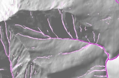
- The flow accumulation threshold value (Table 38) is applied to produce the output derivative. Figure 82 and Figure 83 show examples of D-Infinity flowpaths in conjunction with the previously described geomorphic indices.
D-infinity flow accumulation analysis is available in most GIS Software systems.
| Parameter | Values for Lidar | Values for IfSAR |
| D-infinity flow accumulation threshold for inclusion in GMI | 12500 | 500 |


Multiscale Elevation Percentile
Multiscale elevation percentile derivative (MEP) is a measure of local topographic position (Lindsay, 2018). It is a neighborhood-based algorithm that characterizes the relative vertical position of a cell as a percentile of the local elevation distribution within a range of neighborhood sizes. The 0 percentile is the lowest relative point in the window and 100 percentile is the highest.
The process used to produce the multiscale elevation percentile derivative is as follows:
- Multiscale elevation percentile is performed on the smoothed elevation surface.
- Cells with values less than the maximum percentile (Table 39) are extracted to produce the output derivative. Figure 84 and Figure 85 show examples of MEP in conjunction with the previously described geomorphic indices.
Multiscale elevation percentile is available in Whitebox tools.
| Parameter | Value |
| Number of significant digits used while binning elevation values | 3 |
| Minimum search neighborhood radius in grid cells | 1 |
| Step size as any positive non-zero integer | 1 |
| Number of steps | 10 |
| Step nonlinearity factor | 1 |
| Maximum percentile to include in GMI | 10 |


Geomorphic Index (GMI)
The GMI is created by combining the elevation derivative components into a single value that is more comprehensive than any one technique alone for identifying channelization in an elevation surface.
The process used to produce the GMI is as follows:
- The binary outputs from Multiscale Elevation Percentile, BotHat, valley Geomorphons, and D-infinity flow accumulation are added together.
- Any cells overlapping the binary output from ridge Geomorphons are removed to exclude rises in elevation that may have been captured erroneously by other derivatives.
- If the GMI output contains many isolated sinks or artifacts because of a particularly rough terrain, a de-noise step can be run. This step removes isolated regions of GMI that have a maximum GMI value of 1 (only one geomorphic derivative present) and are less than 1,000 square meters in area.
The resulting GMI contains values from 1 to 4, where 1 represents areas where only 1 derivative component identified potential channelization or conditions that would support hydrography; and 4 represents areas where all 4 derivative components identify potential channelization. Figure 86 and Figure 87 show the output of the GMI process.

Non-breaching and surface-flowing linear features in the elevation-derived hydrography specifications are defined based on whether the flow path is within a channel (Stream/river and Canal/ditch) or outside of a channel (drainageway or indefinite surface connector). The GMI is used to validate the classification of features and to determine whether the horizontal placement of features within channels on the elevation surface is accurate. It is also helpful in identifying areas of potential network omission and proper culvert placement.
The stream network is rasterized and compared to the GMI raster layer during data validation. A feature within a channel (Stream/river or Canal/ditch) is flagged as a potential error if more than 25% of the feature is outside of the GMI. This could indicate that the feature was delineated outside of the channel, or that the feature, or a section of the feature, was misclassified as a Stream/river or Canal/ditch and should be classified as a feature that is not within a channel on the elevation surface. It may also be a commission error; in which case the feature should be removed. An FCode indicating a feature should not be within a channel on the elevation surface is flagged as a potential error if more than 40% of the feature is within GMI values greater than 1. This may indicate that the feature or part of its length was misclassified as a feature within a channel on the elevation surface. Figure 88 shows examples of potentially misaligned vector features identified by analysis against the GMI. Figure 89 shows different scenarios interpreting line features using GMI.


The test for potential omission errors removes the areas in the GMI that contain hydrographic features. Large areas that have a GMI with a value of 2 or more but no vector hydrographic features within them are flagged as potential omission areas. Omission areas that are close to roads are removed to avoid overcollection of ditch networks along transportation features.
Appendix 3 References
Jasiewicz, J and Stepinski, T. J., Geomorphons - a pattern recognition approach to classification and mapping of landforms, Geomorphology, 182, January 15, 2013: 147-56. https://doi.org/10.1016/j.geomorph.2012.11.005https://doi.org/10.1016/j…
Lindsay JB, Francioni A, Cockburn JMH. 2019. LiDAR DEM smoothing and the preservation of drainage features. Remote Sensing, 11(16), 1926; DOI: 10.3390/rs11161926.
Newman, D. R., Lindsay, J. B., and Cockburn, J. M. H. (2018). Evaluating metrics of local topographic position for multiscale geomorphometric analysis. Geomorphology, 312, 40-50.
Rodriguez, F., E. Maire, P. Courjault-Rade, and J. Darrozes. 2002. “The Black Top Hat function applied to a DEM: A tool to estimate recent incision in a mountainous watershed (Estibere Watershed, Central Pyrenees).” Geophysical Research Letters 29(6): 9.1–9.4.
Tarboton, D. G., (1997), "A New Method for the Determination of Flow Directions and Contributing Areas in Grid Digital Elevation Models," Water Resources Research, 33(2): 309-319
U.S. Geological Survey, 2024, 3DEP Spatial Metadata: U.S. Geological Survey webpage, accessed July 2024 at https://www.usgs.gov/3d-elevation-program/3dep-spatial-metadata.
Lindsay, John. (2020). Whitebox User Manual accessed July 2024 at https://www.whiteboxgeo.com/manual/wbt_book/intro.html.