
The Apollo 11 Traverses (left) did not travel more than ~1/10th of a mile from the LEM. The Apollo 17 Traverses (base image), on the other hand, traveled 22.2 miles in Grover. This map illustrates the difference in scale between the two missions. Photo Credit: NASA/GFSC/ASU, USGS Astrogeology
Images
Browse here for some of our available imagery. We may get permission to use some non-USGS images and these should be marked and are subject to copyright laws. USGS Astrogeology images can be freely downloaded.
Filter Total Items: 252

Comparison of Apollo 11 and Apollo 17 traverses
The Apollo 11 Traverses (left) did not travel more than ~1/10th of a mile from the LEM. The Apollo 17 Traverses (base image), on the other hand, traveled 22.2 miles in Grover. This map illustrates the difference in scale between the two missions. Photo Credit: NASA/GFSC/ASU, USGS Astrogeology

Example of nested mapping scales at the Apollo 17 landing site
The nested quality of USGS IMAP 800 is exemplified in this image. The inset of the 1:50K (smaller area, larger scale) landing site map is outlined on the 1:250K (larger area, smaller scale) map of the Taurus Littrow area. Photo Credit: USGS Astrogeology
The nested quality of USGS IMAP 800 is exemplified in this image. The inset of the 1:50K (smaller area, larger scale) landing site map is outlined on the 1:250K (larger area, smaller scale) map of the Taurus Littrow area. Photo Credit: USGS Astrogeology

Hunga Tonga Volcano Ash Plume
GOES-West image of the explosive eruption of the Hunga Tonga volcano in 2022. The explosion atmospheric pressure waves that traveled around the world. Read more here.
GOES-West image of the explosive eruption of the Hunga Tonga volcano in 2022. The explosion atmospheric pressure waves that traveled around the world. Read more here.

Lunar Reconnaissance Orbiter Camera Mosaic of Gruithuisen Domes
Lunar Reconnaissance Orbiter Camera (LROC) mosaic of the Gruithuisen (pronounced “groot-high-sen”) domes on the Moon. These unusual high-silica volcanic features are the target of the NASA Lunar Vulkan Imaging Spectroscopy Explorer (Lunar-VISE) mission. USGS scientist Kristen Bennett is a member of the Lunar-VISE science team.
Lunar Reconnaissance Orbiter Camera (LROC) mosaic of the Gruithuisen (pronounced “groot-high-sen”) domes on the Moon. These unusual high-silica volcanic features are the target of the NASA Lunar Vulkan Imaging Spectroscopy Explorer (Lunar-VISE) mission. USGS scientist Kristen Bennett is a member of the Lunar-VISE science team.

Asteroid Impact Modeling Working Group Hikes into Meteor Crater
This photograph shows members of the Asteroid Impact Modeling Working Group workshop participants descending into Meteor Crater in northern Arizona. Meteor Crater is the best-preserved asteroid impact crater on Earth. It has been used to study the effects of impact, and as a site to train astronauts.
This photograph shows members of the Asteroid Impact Modeling Working Group workshop participants descending into Meteor Crater in northern Arizona. Meteor Crater is the best-preserved asteroid impact crater on Earth. It has been used to study the effects of impact, and as a site to train astronauts.
Python Hyperspectral Analysis Tool (PyHAT) Logo
This a version of the logo for the Python Hyperspectral Analysis Tool (PyHAT). It is intended for use in info boxes on the USGS website. The spectrum in the graphic is a laser induced breakdown spectroscopy spectrum, plotted on a logarithmic y axis to emphasize weaker emission peaks.
This a version of the logo for the Python Hyperspectral Analysis Tool (PyHAT). It is intended for use in info boxes on the USGS website. The spectrum in the graphic is a laser induced breakdown spectroscopy spectrum, plotted on a logarithmic y axis to emphasize weaker emission peaks.
Python Hyperspectral Analysis Tool (PyHAT) Data Format Example
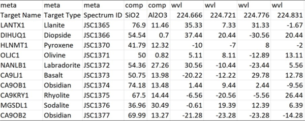
Screenshot showing the simple data format used by the Python Hyperspectral Analysis Tool (PyHAT). Spectra are stored in rows of the table, along with their associated metadata and compositional information.
Screenshot showing the simple data format used by the Python Hyperspectral Analysis Tool (PyHAT). Spectra are stored in rows of the table, along with their associated metadata and compositional information.

MSL image of the Martian Surface on sol 4158
This image was taken of the Martian surface by the NASA MSL rover on sol 4158, showing an assortment of clasts.
This image was taken of the Martian surface by the NASA MSL rover on sol 4158, showing an assortment of clasts.

Python Hyperspectral Analysis Tool (PyHAT) Banner Image
This image is intended as a summary/promotional image for the Python Hyperspectral Analysis Tool (PyHAT) software.
This image is intended as a summary/promotional image for the Python Hyperspectral Analysis Tool (PyHAT) software.
Python Hyperspectral Analysis Tool (PyHAT) Mineral Parameter Map Example - Jezero Crater, Mars
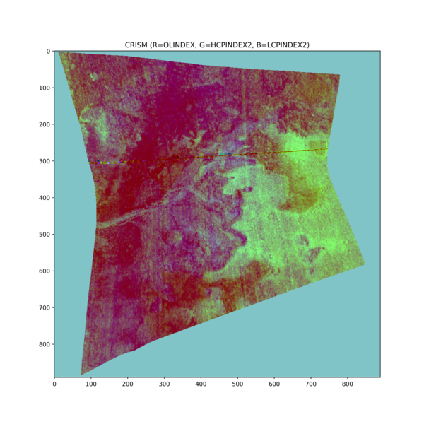
This figure shows an example mineral parameter map image generated using PyHAT. The area in this Compact Reconnaissance Imaging Spectrometer for Mars (CRISM) image is Jezero crater, the landing site of NASA's Mars Perseverance rover.
This figure shows an example mineral parameter map image generated using PyHAT. The area in this Compact Reconnaissance Imaging Spectrometer for Mars (CRISM) image is Jezero crater, the landing site of NASA's Mars Perseverance rover.

NLB_764937797EDR_F1061524NCAM00277M_.jpeg
Image shows a poorly sorted collection of clasts, taken by the NASA Mars Curiosity rover on sol 4139.
Image shows a poorly sorted collection of clasts, taken by the NASA Mars Curiosity rover on sol 4139.
Python Hyperspectral Analysis Tool (PyHAT) Principal Component Analysis (PCA) Plot Example
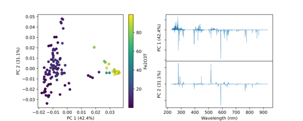
This figure shows an example PCA plot generated using PyHAT. The input data were laser induced breakdown spectroscopy (LIBS) spectra. PyHAT was used to apply a baseline correction and normalization to the total intensity for each spectrum.
This figure shows an example PCA plot generated using PyHAT. The input data were laser induced breakdown spectroscopy (LIBS) spectra. PyHAT was used to apply a baseline correction and normalization to the total intensity for each spectrum.
Python Hyperspectral Analysis Tool (PyHAT) Principal Component Analysis K-Means Clustering Example
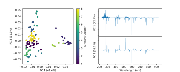
linkThis figure shows an example PCA plot generated using PyHAT. The input data were laser induced breakdown spectroscopy (LIBS) spectra. PyHAT was used to apply a baseline correction and normalization to the total intensity for each spectrum.
Python Hyperspectral Analysis Tool (PyHAT) Principal Component Analysis K-Means Clustering Example
linkThis figure shows an example PCA plot generated using PyHAT. The input data were laser induced breakdown spectroscopy (LIBS) spectra. PyHAT was used to apply a baseline correction and normalization to the total intensity for each spectrum.
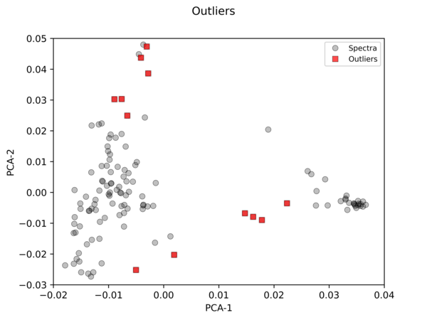
Python Hyperspectral Analysis Tool (PyHAT) Outlier Identification Example
This figure shows an example of outlier identification using PyHAT. The input data were laser induced breakdown spectroscopy (LIBS) spectra. PyHAT was used to apply a baseline correction and normalization to the total intensity for each spectrum. Dimensionality was then reduced using principal components analysis (PCA).
This figure shows an example of outlier identification using PyHAT. The input data were laser induced breakdown spectroscopy (LIBS) spectra. PyHAT was used to apply a baseline correction and normalization to the total intensity for each spectrum. Dimensionality was then reduced using principal components analysis (PCA).
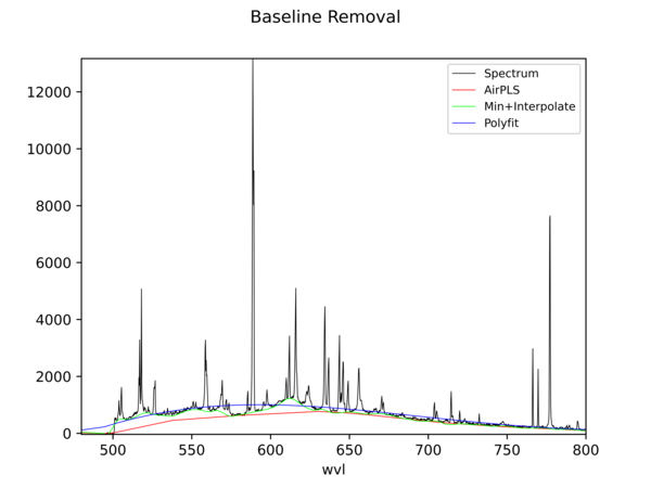
Python Hyperspectral Analysis Tool (PyHAT) Baseline Removal Plot Example
This figure shows an example spectrum plot generated using PyHAT. The black line is a laser induced breakdown spectroscopy (LIBS) spectrum of a basalt sample. The colored lines show the baseline estimated using several different algorithms.
This figure shows an example spectrum plot generated using PyHAT. The black line is a laser induced breakdown spectroscopy (LIBS) spectrum of a basalt sample. The colored lines show the baseline estimated using several different algorithms.
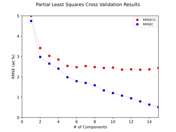
Python Hyperspectral Analysis Tool (PyHAT) Partial Least Squares Cross Validation Example
This figure shows the results of cross-validating a Partial Least Squares (PLS) model to predict the abundance of CaO in geologic targets using PyHAT. Cross validation is necessary to optimize the parameters of a regression algorithm to avoid overfitting.
This figure shows the results of cross-validating a Partial Least Squares (PLS) model to predict the abundance of CaO in geologic targets using PyHAT. Cross validation is necessary to optimize the parameters of a regression algorithm to avoid overfitting.
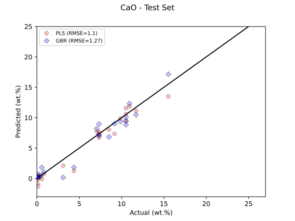
Python Hyperspectral Analysis Tool (PyHAT) Regression Example
This figure compares the results of two regression models to predict the abundance of CaO in geologic standards based on their laser induced breakdown spectroscopy (LIBS) spectra using PyHAT. The horizontal axis is the independently measured CaO abundance, the vertical axis is the abundance predicted by the models.
This figure compares the results of two regression models to predict the abundance of CaO in geologic standards based on their laser induced breakdown spectroscopy (LIBS) spectra using PyHAT. The horizontal axis is the independently measured CaO abundance, the vertical axis is the abundance predicted by the models.
PyHAT Thumbnail
This is the small logo for the Python Hyperspectral Analysis Tool (PyHAT). It is intended for use as a thumbnail. The spectrum in the graphic is a laser induced breakdown spectroscopy spectrum, plotted on a logarithmic y axis to emphasize weaker emission peaks.
This is the small logo for the Python Hyperspectral Analysis Tool (PyHAT). It is intended for use as a thumbnail. The spectrum in the graphic is a laser induced breakdown spectroscopy spectrum, plotted on a logarithmic y axis to emphasize weaker emission peaks.

Grover Coloring Page
A coloring page and information about Grover, the USGS's geologic rover that went to the moon during the Apollo missions.
A coloring page and information about Grover, the USGS's geologic rover that went to the moon during the Apollo missions.

Screenshot GeoSTAC project.png
Screenshot of the user interface of the GeoSTAC project, with symbolized polygons on a Mars map (left) and a selection panel (right).
Screenshot of the user interface of the GeoSTAC project, with symbolized polygons on a Mars map (left) and a selection panel (right).

Photo of the GeoKings team.png
Photo of the GeoKings team taken by mentor Trent Hare in a ballroom full of other people, which is the poster session where they won their award. GeoKings from left to right: Zack Bryant, Jackson Brittain, John Cardeccia, Andrew Usvat, and Alex Poole.
Photo of the GeoKings team taken by mentor Trent Hare in a ballroom full of other people, which is the poster session where they won their award. GeoKings from left to right: Zack Bryant, Jackson Brittain, John Cardeccia, Andrew Usvat, and Alex Poole.